In this blog, we start with a qualitative overview of the small-world effect, also known as the “six degrees of separation,” followed by a quantitative analysis using computational methods, and finally, a description of the phenomenon through the framework of phase transitions and critical phenomena. From the surface level to deeper insights, I aim to explore the mechanics underlying this phenomenon and how this understanding can be extended to other large-scale phenomena.
Six Degree of Separation: An Inquiry into Social Cloesness
If you know six people, preferably from different parts of the world in addition to your closest acquanintances, you can effectively connect to everyone on the planet. This concept, known as “six degrees of separation,” was first introduced by novelist Frigyes Karinthy. It describes the significant reduction in social distance when a few shortcuts are added in a social network. Below is a YouTube video by the youtuber Veritasium that introduces this idea (where I first learned about the concept of six degrees of separation).
However, it mains as a qualitative thought in 1922 because computation and math theory is not available to quantify this social occurence.
It wasn’t until 1998 that Duncan J. Watts and Steven H. Strogatz introduced a random graph procedure to study this effect quantitatively. ( Citation: 1998 Watts, D. & Strogatz, S. (1998). Collective dynamics of “small-world” networks. Nature, 393(6684). 440–442. https://doi.org/10.1038/30918 )
Networkx Simulation on Random Graphs
The method involves generating a network (or graph interchangeably) with \(L\) nodes. The nearest neighbors of each node are well-defined: we arrange the nodes in a circle and connect them to their nearest neighbors, determined by the parameter \(Z\) (an even number for evenly distributed connections). To illustrate the procedure, below is a graph with \(N = 20\) and \(Z = 4\). The graph is generated using NetworkX, an extensive Python library for network theory.
import matplotlib.pyplot as plt
import networkx as nx
L = 20
Z = 4
p = 0
G = nx.newman_watts_strogatz_graph(L, Z, p)
nx.draw(G, pos=nx.circular_layout(G))
plt.draw()
plt.savefig("simple_graph.png")
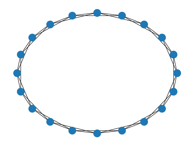
This is a simple connected network with 20 nodes, 4 nearest neighbors, and no shortcuts.
Adding Shortcuts
Now, how quickly we can travel from one point on the graph to another depends on the shortest path. By randomly rewiring the existing connections \(Lkp\) shortcuts between unconnected nodes, we can reduce the shortest travel distance. We characterize the connectivity by the average shortest distance (l) of the graph. The algorithm to calculate the graph’s average distance is as follows:
Start from node \(L_{i}\) and measure the distance \(d\) to the nearest neighbors.
Accumulate these distances, move on to those nearest neighbors, and repeat step 1 until all nodes are exhausted.
Divide the cummulative distance by the total neighbor of \(L_{i}\) and yields the average distance of node \(L_{i}\)
Repeat step 1 for the next nodes \(N_{i+1}\) until all nodes exhaust
Sum up the average distance of each nodes and divided by the number of nodes
Effects of shortcuts on the Average Shortest Path Length
NetworkX has an optimized built-in function to calculate the graph’s shortest distance, so we’ll use that. After we know the quantitative measurement of the separation distance, we rewired the existing edges probabilistically by \(p\). (Though we keep those wires being rewired to avoid disconnected component) On average, \( p L k \) shortcuts are added to the graph, where we defined \(k\) to be \(k = \frac{Z}{2}\). Next, we illustrate the network qualitatively with different parameters. For a sparsely connected graph and a densely populated graph they are topologically very different from each other:
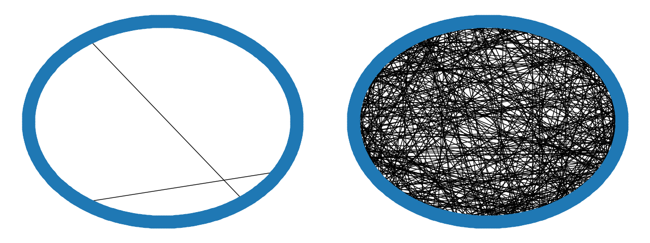
Qualitatively, a graph could be sparse or dense depending on the number of shortcuts. For network of \(L=500, k = 2\). The left graph is produced by \(p=0.001\) and the right graph is produced by \(p = 0.1\)
For the sparse graph above, the average seperation can go up to \(23\). Whereas for the densely populated graph, the distance of separation reduces to about \(4\).
So, the six degree of separation makes qualitative sense as observe from the above figure. Next, we want to know how adding the shortcuts will impact the average shortest path \(l\). To do this, we vary \( p \) from \(0.001 \) to \( 0.1 \) for a graph with \(50\) nodes, nearest neighbor connection \(Z = 2\). Plotting the result:
N = 50
Z = 2
p = np.linspace(0.001, 1, 100)

distance_distribution = []
for s in p:
    G = nx.newman_watts_strogatz_graph(N, Z, s)
    avg_shortest_path = nx.average_shortest_path_length(G)
    distance_distribution.append(avg_shortest_path)

fig,ax = plt.subplots()
ax.scatter(p, distance_distribution)
ax.set_ylabel("Separation")
ax.set_xlabel("p")
ax.set_title("Small-world effects")
plt.savefig("small_world.png")
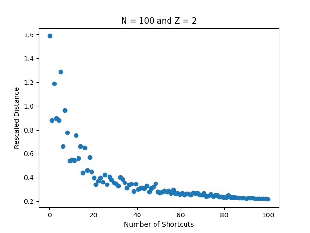
As \(p\) increases, the number of shortcuts \(Lpk\) also increases, which reduce the shortest distance with a scaling law as shown.
We observe a dramatic decrease in the average separation (s) in the small (p) region. Around (s = 6), the curve shifts sharply, transitioning from a drastic decrease to asymptotic behavior towards zero separation. From our computer simulation and calculations, we elaborate the vague conclusion from social science to a firm numerical justification. In what follows, we want to understand this phenomena with renormalization group, a model that studies critical behavior of systems.
Renormalization Group Analysis of Random Graph
In the renormalization group approach to this random network model, the transition from a regular graph to a random graph at \(p = 0\) can be treated as a continuous phase transition. Following this perspective, we refer to the work of ( Citation: 1999 Newman, M. & Watts, D. (1999). Renormalization group analysis of the small-world network model. Physics Letters A, 263(4–6). 341–346. https://doi.org/10.1016/s0375-9601(99)00757-4 ) to elaborate on the scaling scheme used to derive the scaling exponent \(\tau = 1\) in the form \(\xi \propto p^{-\tau}\), where \(\xi\) is analogous to the correlation length in a typical physical system.
Before diving into the technical details, we first ask the following questions:
- What kind of question we want to answer in this small world model?
The six degrees of separation and the scaling graph suggest an analytic form that relates the shortest path length to system variables. However, it’s difficult to derive this form because the shortest path length is calculated via a computational routine, and no analytic form can be derived from the algorithm.
- Why is the renormalization group method a good candidate for solving this small-world problem?
The renormalization group studies the scaling behavior of systems near critical points, where the correlation length governs the entire system’s behavior. The small-world model demonstrates two regimes of behavior, suggesting a transition and a critical point. This motivates mapping the small-world problem to a phase transition problem.
Two regimes of behavior
In the first regime of phase, the average distance scales linear with the size of the graph \(L\) because the only way to reach other nodes is by traversing through the neighbors.
The other regime is the random graph region, where the average distance scales approximately as lograithm of \(L\).
Between these two regimes, the graph undergoes critical behavior at \(p=0\) for a system size \(L=\xi\), where the number of shortcuts approximately be \(Lk\xi \approx 1\). Here, \(\xi\) is analogous to the correlation length in a typical physical system, which diverges at the critical point. For \(pk\xi \approx 1\) to hold at \(p\rightarrow 1\), \(\xi\) must goes to infinity at the critical point.
To better understand the concept of correlation length in a typical physical system, note that a continuous phase transition involves moving from a disordered state to an ordered state as a relevant parameter decreases. As the system approaches this transition, the correlation length, which measures the collective order, increases. At the critical region, the correlation length becomes very large because order tends to align throughout the system.
It is this diverging behavior of the correlation length near the critical point that allows us to formulate an analytic scaling relation between system parameters, enabling us to solve the small-world model using the renormalization group (RG) method.
Parameters of the system: Scaling form
For those interested in learning more about the RG method and the justification for diverging correlation lengths dominating the behavior of continuous phase transitions, see ( Citation: Hohenberg & Halperin, 1977, pp. 9-12 Hohenberg, P. & Halperin, B. (1977). Theory of dynamic critical phenomena. Rev. Mod. Phys., 49. 435–479. https://doi.org/10.1103/RevModPhys.49.435 ) . This work also explains how scaling effectively removes irrelevant degrees of freedom from the system. This process reduces the degrees of freedom, bringing the system to a different one with a different correlation length. Except at the critical point—where the correlation length is infinite and remains unchanged under scaling—the scaling law relates systems with different correlation lengths. If this leads to a simplified solvable model, meaningful conclusions can be drawn about the complex system that we started with.
In our case, the regular graph region has zero shortcuts, while the random graph has more than one. Therefore, we expect the transition to occur when the first shortcut appears, \(\xi kp \approx 1\) where \(\xi = L\) at some system size.
Assuming homogeneity leads to the scaling form of the correlation length, with the relevant system parameters following a scaling form for a function \(f(x, y)\) that satisfies homogeneous:
$$ f(x, y) = x^{\lambda} g\left(\frac{y}{x^{\mu}}\right) $$
This is further discussed in ( Citation: Toulouse & Pfeuty, 1977 Toulouse, G. & Pfeuty, P. (1977). Introduction to the renormalization group and to critical phenomena. Wiley. )
n our problem, the only relevant length scales are the average shortest path length \(\xi\) and the number of nodes \(L\). Based on the assumptions in Newman’s paper, we obtain the following scaling equation:
$$ l = L f\left(\frac{L}{\xi} \right) $$
Alternatively, assuming \(\xi \propto p^{-\tau}\):
$$ l = L f\left(L p^{-\tau} \right) $$
We propose a scaling procedure where \(L^{\prime} = \frac{1}{2}L \), reducing the system by half, and \(p^{\prime} = 2p\), keeping the number of shortcuts \(Lkp\) unchanged.
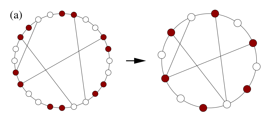
Grouping procedure proposed by Newman and Watts. Dot with the same color are merged by scaling.
Comparing the ratio \(\frac{l^{\prime}}{l}\) and solvig for \(\tau\) we find:
$$ \tau = \frac{\log{(L/L^{\prime})}}{\log{(p^{\prime}/p)}} = 1$$
Reaching the result \(\tau =1 \) requires significant work, including making educated assumptions about the model. After all, the small-world model is not governed by simple universal laws but by collective behavior that blurs microscopic details. Newman and Watts verified the exponent \(\tau = 1\) through extensive numerical experiments. They also compared the system’s behavior if the exponent was \(\tau = \frac{2}{3}\), derived from an alternative RG approach but yielding less accurate results.
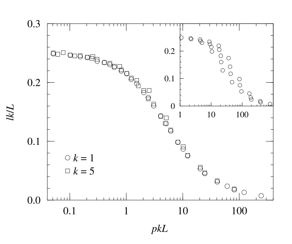
The scaling behavior for \(k = 1\) and \(k =5\). For \(\tau = \frac{2}{3}\) is also tested in the top-right corner of the figure
For \(k > 1\), the authors adopted a different coarse-graining approach to handle computational limitations, but the same exponent was obtained. As an extension, they also derived the scaling and exponent for systems with higher dimensions. For interested readers, detailed derivations can be found in the paper ( Citation: 1999 Newman, M. & Watts, D. (1999). Renormalization group analysis of the small-world network model. Physics Letters A, 263(4–6). 341–346. https://doi.org/10.1016/s0375-9601(99)00757-4 )
Remarks
In this blog, we have revisited the arguments from Newman and Watts’ paper, reinterpreting them within the framework of phase transitions. Along the way, we provided additional physical insights and explanations for steps that were either implicit or assumed in the original work.
To understand complex phenomena through the lens of phase transitions and the renormalization group (RG), it is crucial to first identify the distinct regimes of behavior, where the system’s qualitative properties change significantly. These transitions are marked by changes in symmetry—something that, according to condensed matter physics, cannot occur gradually. This is why conventional methods like perturbation theory are inadequate in such cases. Instead, a scaling law must be derived, capturing the relevant parameters at the critical point.
However, deriving this scaling law involves substantial numerical work and carefully made assumptions. In our application of the RG method, we focused on the scaling form to extract the exponent, yet the deeper physical meaning of the RG flow itself remains somewhat elusive.
The true power of the RG method lies in its ability to connect systems that, despite appearing different, share the same critical behavior as they approach a diverging correlation length. This ability to group systems by their underlying topological structure is a key strength of the RG approach, but was not entirely clear how this aspect of the RG approach plays in the application on the small-world model.
Reference
- Newman & Watts (1999)
- Newman, M. & Watts, D. (1999). Renormalization group analysis of the small-world network model. Physics Letters A, 263(4–6). 341–346. https://doi.org/10.1016/s0375-9601(99)00757-4
- Hohenberg & Halperin (1977)
- Hohenberg, P. & Halperin, B. (1977). Theory of dynamic critical phenomena. Rev. Mod. Phys., 49. 435–479. https://doi.org/10.1103/RevModPhys.49.435
- Toulouse & Pfeuty (1977)
- Toulouse, G. & Pfeuty, P. (1977). Introduction to the renormalization group and to critical phenomena. Wiley.
- Watts & Strogatz (1998)
- Watts, D. & Strogatz, S. (1998). Collective dynamics of “small-world” networks. Nature, 393(6684). 440–442. https://doi.org/10.1038/30918