Renormalization Group: A Descriptive Overview

Renormalization Group Approach in Dynamical System

The renormalization group (RG) method is an approximation technique initially developed for solving strongly interacting many-body problems in quantum field theory, where perturbative solutions deviate from the actual solutions. The fundamental concept of the renormalization group approach is to eliminate irrelevant degrees of freedom in a physical system while preserving its essential characteristics ( Citation: P. Kopietz, 2010 P. Kopietz, F. (2010). Introduction to the Functional Renormalization Group (1). Springer, Berlin Heidelberg 2010. https://doi.org/10.1007/978-3-642-05094-7 ) . This method has been extended to the field of statistical mechanics, providing a quantitative description of universality and scale invariance phenomena.

Universality and Scale Invariance

Universality refers to the observation that distinct physical systems can exhibit similar behavior near their critical points. Scale invariance occurs when the qualitative features of a system remain unchanged as we vary the system’s size ( Citation: Sethna, 2020 Sethna, J. (2020). Entropy, Order Parameters, and Complexity (2). Clarendon Press. ) . These concepts offer a framework for categorizing phenomena that exhibit self-replicating patterns in space (fractal structures) and time (period doubling). In this review, we will explore the relationship between changing the scale of a system and the emergence of chaos at certain parameter limits. By applying the renormalization group method, we can establish the close connection between these concepts and provide a unifying language for their analysis.

Renormalization Procedure: Decimation and Rescaling

The renormalization group method involves two key steps: decimation (mode reduction) and rescaling. Decimation eliminates irrelevant degrees of freedom in the system, while rescaling ensures that the remaining parameters are adjusted in such a way that the essential properties of the system are preserved.

We can describe the action of the renormalization group on a system using the operator \(R(b;g)\), where $g$ represents the relevant parameters or coupling terms that describe the system, and \(b\) defines the scaling operation. By applying this operator recursively, we can track the evolution of the parameters \(g\) as we scale the system by a factor of \(b\).

$$ \vec{g}^{\prime} = \vec{R}(b;\vec{g}) $$ $$ \vec{g}^{\prime\prime} = \vec{R}(b^{\prime};\vec{g}^{\prime}) = \vec{R}(b^{\prime};\vec{R}(b;\vec{g})) = \vec{R}(b^{\prime}b;\vec{g}^{\prime}) $$

By repeatedly applying this operation $n$ times, we obtain the relationship:

$$ \vec{g}^{(n)} = \vec{R}(b;\vec{g})^{n-1}=\vec{R}(b^{(n)};\vec{g}) $$

This equation signifies that by removing irrelevant degrees of freedom, we modify the system’s coupling parameters \(\vec{g}\). To ensure that \(\vec{g}\) remains fixed at each iteration, the scaling operation $b$ must be recursively applied.

The conceptual understanding of the renormalization group method is straightforward, but the challenge lies in determining the form of the operator \(\vec{R}(b;\vec{g})\), as we will see in the case of the logistic map.

Example I: One-dimensional Ising Model

In the case of one dimension Ising model, every resursive process scales the total number of lattice by \( \frac{1}{2} \) while keeping the form of partition function fixed. As a result, the coupling constant \( g \equiv \frac{J}{T} \) is mapped to \( g^{\prime} \) accordingly to match the partition function.

By scaling the lattice point by half, the transfer matrix is rescaled as such

$$ T^{\prime}=e^{f^{\prime}}[[e^{g^{\prime}+h^{\prime}}, e^{-g^{\prime}}], [e^{-g^{\prime}}, E^{g^{\prime} - h^{\prime}}]] = e^{2f}[e^{2g+2h} + e^{-2g}] $$

Which gives us three equations to solve for the three new coupling constant in terms of the old coupling constant. Writting out explicitly.

• The renormalized external magnetic field $$ h^{\prime} = h + \frac{1}{2}\ln{\left[ \frac{\cosh{(2g+h)}}{\cosh{2g-h}} \right]} $$

In the absent of external magnetic field

• The renormalized free energy $$ f^{\prime} = 2f + + \ln{\left( 2 \sqrt{2\cosh{2g}} \right)} $$

• The renormalized nearest-neighbor interaction $$ \tanh{g^{\prime}} = \tanh^{2}g $$

• The RG flow and fixed points

Defining \( x_{0} \) to be

$$ x_{0} = \tanh{\left( \frac{J}{T} \right)} = \tanh{g} $$

which follows that

$$ \tanh{g_{1}} = x_{1} = x_{0}^{2} $$

And we obtain the recursion relation of the fraction \( g \)

$$ x_{n+1} = x_{n}^{2} $$ $$ x_{n} = \tanh{\left( \frac{J}{T_{n}} \right)} $$

Since hyperbolic tangent is asmptotic to -1 and +1, hence the recursion will map the hyperbolic tangent from \( |1| \) to \( 0 \), or zero temperature to infinite temperature as we shrinks the system.

Alternatively, the RG flow could be captured by calculating the correlation function \( G(r_{i} - r_{j}) \) and the correlation length \( \xi \). Recall that \( \xi \) is defined in terms of the asymptotic behavor of the correlation function \( G(r_{i} - r_{j}) \) for \( |r_{i} - r_{j}| \rightarrow \infty \), or, equivalently, in terms of the behavior of its Fourier transfrom \( G(k) \) for small wave vectors.

$$ \xi^{\prime} \equiv \xi (x^{\prime}) = \frac{\xi (x)}{b} $$

$$ \xi (x^{2}) = \frac{\xi (x)}{2} $$

$$ \xi (x) = - \frac{a_{0}}{\ln{x}} $$

Hence

$$ \xi \sim \frac{a}{2} e^{2J/T} $$

Example II: Logistic Map and Period Doubling

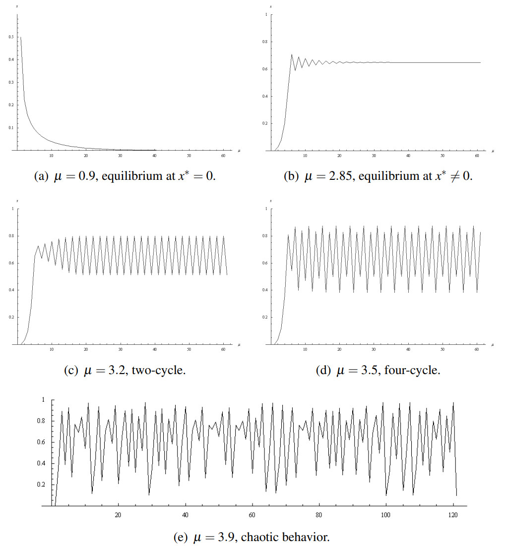
The logistic map is an example of a discrete-time dynamical system defined by the recursion law:

$$ x_{n+1} = f(x_{n})=\mu x (1-x) $$

Although the equation appears simple, it exhibits a captivating phenomenon known as period doubling as the bifurcation parameter $\mu$ increases, ultimately leading to chaos at the limit $\mu_{\infty}$, as illustrated in Figure below.

Interestingly, a constant $\delta$ known as the Feigenbaum constant emerges and remains fixed across certain families of functions. It can be stated as in the limit of $n \rightarrow \infty$

$$ \delta = \lim_{n\rightarrow \infty} \frac{\mu_{n}-\mu_{n-1}}{\mu_{n+1}-\mu_{n}} $$

Through numerical analysis, the Feigenbaum constant has been calculated to be a value close to $4.66914$.

The RG method provides a quantitative approach to calculating the Feigenbaum constant and generalizing the behavior of period doubling phenomena to a function space. However, the mathematical derivations involved can be complex, and interested readers are encouraged to consult relevant papers ( Citation: Sfondrini, 2012 Sfondrini, A. (2012). Introduction to universality and renormalization group techniques. Retrieved from http://arxiv.org/abs/1210.2262 ) for more detailed information.

To keep it simple, we will only be focusing on providing a descriptive account of the steps involved in calculating the Feigenbaum constant, with the emphasis on the interpretation of the results and their significance in the dynamical analysis of chaos.

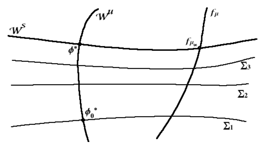
To summarize the steps, we first make observations about the logistic map, recognizing it as a unimodal function. We also note that other unimodal functions exhibit period doubling behavior. We define a functional subspace of unimodal functions and seek to apply the RG method in a way that preserves this characteristic of being unimodel. Once we have the form of \(R(b;g)\) at hand, we evaluate the behavior of the fixed point \(R(\phi^{ast})=\phi^{ast}\) where $\phi$ denotes the flow. Intuitively, we expect to find one unstable manifold with eigenvalues of modulus greater than one that correspond to bifurcation variable \(\mu_{\infty}\) that destabilizes the orbit. And an infinite stable manifold with eigenvalues of modulus less than one corresponds to \(mu_{n}\) that corresponds to stable oribit with period \(2^{n}\). By visualizing the mathematical spaces (refer to the figure below), we can observe that they share similar features with period doubling, albeit in different domains. The spacing of the stable and unstable manifolds follows a geometric series, defining the Feigenbaum constant. By making suitable ansatz for the sequence and fitting it with \(R(\phi)\), we are able to calculate \(\sigma=4.66914\).

This derivation clarifies some confusions and provides a unique perspective on the period doubling phenomenon. It demonstrates how the logistic map, initially perceived as a one-dimensional system that cannot exhibit chaotic behavior, actually resides in an infinite-dimensional space that converges to chaos. Moreover, it reveals that unimodal mapping is the underlying universality group characterized by the Feigenbaum constant, with the logistic map representing just one special case. In simpler derivations, numerical mappings of one set of \(\phi_{n}$ to $\phi_{n-1}\)inform us of the functional form of the renormalization group operator \(R(\phi)=-ag(g(-z/a))\). Without making further assumptions, this form also enables the calculation of the Feigenbaum constant. In this sense, the renormalization group operator captures the essential structure of the onset of chaos behavior.

Bibliography