Site and bond percolation models exhibit a phase transition at a shared critical point, where both demonstrate self-similarity and scale invariance—hallmarks of continuous phase transitions. Using the Renormalization Group (RG) method in ( Citation: Sethna, 2020 Sethna, J. (2020). Entropy, Order Parameters, and Complexity (2). Clarendon Press. ) , which proposed a scaling procedure from the assumption of self-similar, we derive the scaling exponents for the percolation universality class. While this top-down approach offers pedagogical simplicity, it lacks the physical intuition provided by the Ginzburg-Landau framework. To bridge this gap, we explore a cross-referenced analysis of these two approaches, aiming to deepen our understanding of network percolation phenomena.
Introduction
Percolation theory studies the connected compoents of a damaged graph \(G=(V, E)\), where \(V\) denotes the number of nodes and \(E\) denotes the number of edges. The damaging process is done by removing the edges with probability \(p\) - this is called bond percolation - Or removing the nodes with probability \(p\) - this is called site percolation.
The percolation process is closely related to the continuous phase transition discussed in statistical mechanics. One physical example of percolation is the sharpe drop of electrical conductivity as one punches holes on a metal sheet to its critical value. ( Citation: Last & Thouless, 1971 Last, B. & Thouless, D. (1971). Percolation theory and electrical conductivity. Phys. Rev. Lett., 27. 1719–1721. https://doi.org/10.1103/PhysRevLett.27.1719 ) The conductivity of the metal sheet can be written as a function of the area of the holes and it embodies continuous change of physical behavior.
Consider having a few holes to a intact sheet. Current could always find ways to go around the holes featuring the conducting regime. As the number of holes increases to the critical value, the allowed conduction path narrowed down, and eventually the metal sheet falls apart and become fully disconnected. The conductivity varies continuously as area of the holes are being punched through, meanwhile also exhibit two regimes of behavior as the parameter is varied. This experimental set-up is analogous to a percolation problem.
Percolation does not limit to a particular physical phenomena. In fact, it is a common trait of many network system. For example, when modelling the spread of forest fire and infectious diseases ( Citation: Stauffer & Aharony, 1994 Stauffer, D. & Aharony, A. (1994). Introduction to percolation theory. Taylor & Francis. ) , percolation transitions are frequently observed. So, it will be convinient to have a simple random graph model to solely study the percolation effect. In this brief review, we will be considering two dimensional bond percolation and site percolation from a top-down approach. We simulate the model and quantify the observables to derive the scaling law at and near the critical point. Then, we will be justifying some of the observation under the framework of Ginzburg-Landau Equation.
Experiment Set-up
Network Simulation
In a bond percolation network, we initialize a fully connected \(L \times L\) grid lattice and enforcing the periodic boundary condition. Each bond would have probability \(p\) to be removed or equivalently having \(1- p\) probability to be added. For a site percolation, we initialze the graph on a fully connected triangular \(L \times L\) lattice. Though this time we are removing the site instead of the bond.
import main

# Plot a grid network with dimension m x n. Edges have 0.5 probability to be removed

m, n, p = 20, 20, 0.5
main.plot_grid_clusters(m, n, p)

# Plot a grid network with dimension m x m. Edges have 0.5 probability to be removed

# By construction the triangular graph must have L x 2L to be have equivalent sites as the grid network

m, n, p = 20, 40, 0.5
G = main.triangular_percolation(m, n, p)
main.plot_triangular_cluster(G, m, n)
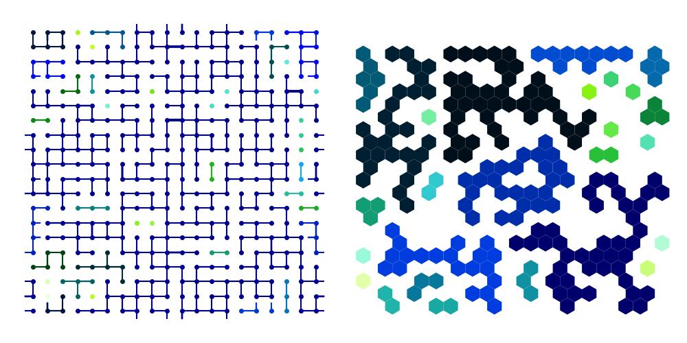
On the left of the graph shows the bond percolation, where each bond between the nodes have probability \(p=1/2\) to be removed. On the right shows the site percolation with the same probability \(p=1/2\). Components of the graph is color coded by their relative size. The larger cluster tend to have a darker color.
As observe from the figure above, the system parameters to control the percolation are the same (the same lattice size \(L\) and probability of removal \(p\)), the microscopic detail, such as the number of nearest neighbor, is different. For the bond percolation, each node has four nearest neighbor whereas for site percolation, each node has six nearest neighbor.
Phases near the critical point
How do we tell that these model exhibit phase transition? To answer this question, we investigate the observables of the graph, such as the distribution of the size of the network components \(n(S)\), where \(S\) refers to the size of the component. As well as the normalized largest components for ensembles with \(P(p) = S_{largest}(p)/L^{2}\), where \(S_{largest}\) representing the largest cluster as a function of the probability \(p\).
We distinguish different phases by the change of symmetry of the system in interest, which often manifest itself through the scaling law of the observables near the criticla point. For example, the melting of ice exhibit a broken translation symmetries changing from liquid to solid. Symmetry, as we know it, cannot change smoothly ( Citation: Anderson, 2019 Anderson, P. (2019). Basic notions of condensed matter physics. Taylor & Francis Limited. ) . Hence, the observables will have a sharp transition, known as scaling, that separate two regimes of behavior.
- Two regimes of behavior
To see that the two regimes of behavior exhibit, we take the limit of these observables as \(p\) ranging from \(0\) to \(1\). At \(p\rightarrow 0\), it is a fully connected graph with \(P(p) = 1\) and \(n(S)= \delta_{S=L\times L}L \times L\). As \(p \rightarrow 1\), it will become a sparsely connected graph and the corresponding \(P(p) = 0\) and \(n(S) = 1\) in the large \(L\) limit.
However, checking the limits will only tell us that the system exhibit two regimes of behavior but necessarily tell us that there must be a critical point separating the two phases. How do we know that there indeed exists a critical point at the phase transition but not some smooth varying function that changes polynomial with \(p\), such as \(P(p) \propto (1-p) \). In general, it is fairly difficult to come up with the analytic form of the observables, and in the case of percolation, it is impossible to have analytic form of the function that covers the entire domain. However, it is possible to derive the behavior near the critical point using the method of Renormalization Group (RG) to approximate the critical behavior. As promosed, from a top-down approach, we would rely on numerical simulation to decide the existence of phases, and then justify the use of RG approach.
- Numerical simulation
Running simulation with \(L = 20\) for different probability \(p\) and comparing the distribution. One will find that the grid percolation has a sharp transition about the critical point \(p_{c} \sim 0.5\). Plotting the grid percolation near the critical point:
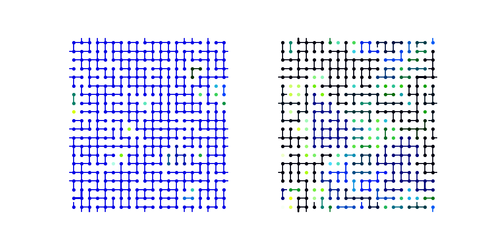
For \(p < 0.5\), as shown for the bond percolation on the left figure, the largest cluster nearly covers the entire graph showing a phase with large \(P(p=0.4)\) value. In constrast, at \(p > 0.5\) as shown on the right figure, clusters broken down in smaller proportion, showing a distinct phase with much smaller \(P(p=0.6)\) value. Even as we close up the difference to the critica value of \(0.5\), these two phases persist, which validates our claim about the system having a critical point at \(p_{c}=0.5\) through a numerical method.
On contrast, we could derive the value of transition if we assume the system must exhibit a critical point where the system drastically changes its behavior. Suppose grid network \(A\) percolates at \(p_{c}\) for \(p_{c} \in (0, 1) \). We could always construct an dual grid network \(B\) by shifting all the nodes to the diagonal and re-connect the nodes where there isn’t any connection in \(A\). The two graph is complementary by construction. So, \(p_{A} = 1- p_{B}\). In addition, both model is statistically equivalent, that implies both network percolate at the same critical value \(p_{c}\). Hence, \(p_{c} = 1 - p_{c}\), yielding the critical value at \(p_{c} = \frac{1}{2}\).
Scaling-law Behavior about the critical point
Right at the critical points, it becomes increasingly difficult to tell the phases of the system. However, there are some interesting observation that could help us get started in the analysis of criticallity.
For the largest cluster with the simulation running at \(L = 1024\) and \(p = 0.5\), no matter if we running with grid or triangular lattice, it displays roughly the same pattern. This is known as universality. In the thermodynamics limit, the macroscopic observables are incensitive to the microscopic detail; the microscopic details behave as a fluctuation that goes away when summed over a large system size.
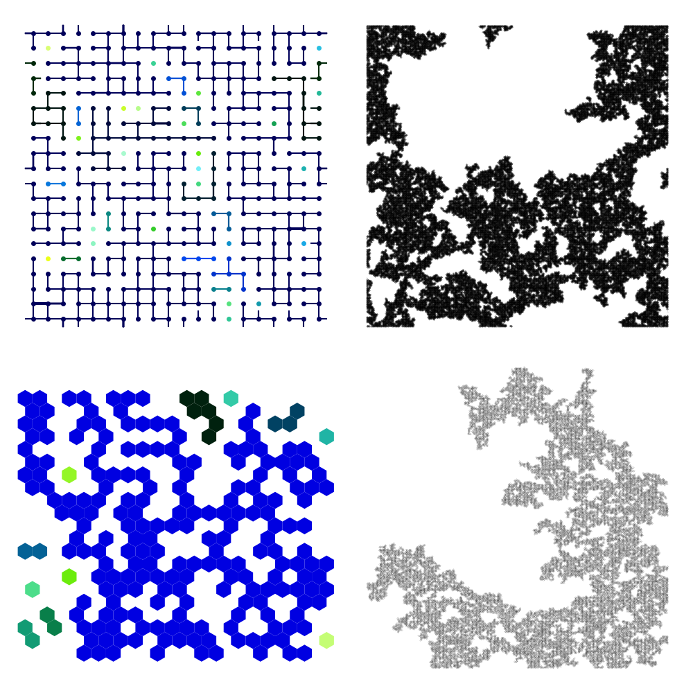
One the left column, we have bond percolation(top) and edge percolation(bottom) at a relatively small system size of \(L = 20\). On the right column, we have the largest cluster from the corresponding bond percolation(top) and edge percolation(bottom) at a much larger system size with \(L = 1024\). Though differed in their density in the large system limit, both models are statistically similar, demonstrating universality.
To quantify the pattern that we are seeing, we propose a coarse grain procedure and it goes as follow: we average over the pixel values of four lattices in squre and replacing the four lattices with a larger square with the average of the four, essentially shrinking the lattice from a size of \(1024 \times 1024\) to \(256 \times 256\); the coarse grained figure remain statistically equivalent. This is known as self similar and scale invariance, two well known features of continuous phase transition.
Power-law at \(p_{c}\)
It is precisely from the observation of self-similar of the system at a large size limit that motivates the top-down derivation of the scaling-law in the percolation network.
Under coarse graining, we will be measuring every observables of the system with a new length scale. Self-similar thus refering to the invariant of the distribution under the change of length scale.
Let \(D(S)\) be the distribution of the cluster with size \(S\). The statement of scale invariance then can be expressed as:
$$D^{\prime}(S) = D(S)$$
where \(D \rightarrow D^{\prime}\) refering to the change of length scale. And hence, the functional of \(D\) has no explicit dependent on \(l\):
$$\partial D / \partial l = 0$$
$$ \frac{dD}{dl} = \frac{\partial D}{\partial S} \frac{dS}{dl} + \frac{\partial D}{\partial l} = \frac{\partial D}{\partial S} \frac{dS}{dl}$$
This is precisely the embodiment of self-similar in the spatial distribution, also known as the fixed point of the RG flow in the parameter space.
How about the functional dependent of of the distribution \(D(S)\) on the size of the distribution \(S\) under rescaling? Since the cluster size \(S\) is dependent on the length scale of the system. Under coarse graining it will be scaled down by some factor \(C = 1 + cdl\).
$$ S^{\prime} = S/C = S/(1+cdl) \approx S-cSdl$$ $$ S^{\prime} - S = dS = -cSdl $$ $$ dS/dl=-cS $$
Consequently, measuring the distribution with coarse grained cluster size will have the following form:
$$ D^{\prime}(S^{\prime}) = D(S^{\prime}) = D(S- cSdl) = D(S + \frac{dS}{dl} dl)=D(S)+\frac{d D}{d S}dS$$
When the cluster gets smaller, the number of cluster will surely increase, requiring \(D(S^{\prime})\) to scale positively with some factor \(A = 1+ adl\).
$$D(S^{\prime}) = AD(S) = D(S)(1+adl) = D(S) + aDdl$$
Equating the two equations above to give:
$$ \frac{dD}{dS}dS = a Ddl $$
Rearanging to remove the dependence on \(dl\) and define \(\tau = \frac{a}{c}\): $$ \frac{dD}{D} = -\frac{a}{c}\frac{dS}{S} $$
$$ D(S) \propto S^{-a/c} = S^{-\tau} $$
The distribution follows a scale-free dependent on the size of the cluster with exponent \(\tau = a/c\). Testing the scaling relation with the theoretical exponent of \(\beta = 187/91\)
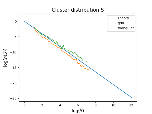
The fluctuation on the experimental value is due to the finite size of the experiment. Each interval of \(\delta S\) is binned. If there is insufficient samples, sometimes it will be gapped like shown on the graph above. But it is obvious that overall trend fluctuatues around the theoretical predicted value which indeed proves the claims that the distribution follows a power-law scaling (showing a straight line on a log-log plot). Noting that both grid percolation and triangular percolation do indeed from the same universality class; they have the same exponent at the critical region.
Power-law near \(p_{c}\)
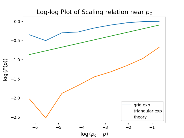
Not only the distribution of the cluster size follow the power-law, the quantity \(P(p)\) as the function of \(p\) also follows a power-law. We could go through the similar derivation of scaling and yield the following relation:
$$ P(p) \sim (p- p_{c})^{\beta} $$
However, if we plot the actual distriubtion, the scaling exponent is quite off from the theoretical value of \(\beta = 5/36\). What is going on?
Qualitatively, a graph could be sparse or dense depending on the number of shortcuts. For network of \(L=500, k = 2\). The left graph is produced by \(p=0.001\) and the right graph is produced by \(p = 0.1\)
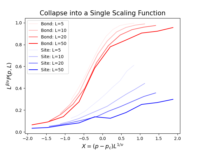
This is because the model is not exactly in the thermodynamics limit. The phase transition and the scaling-law is well-defined only when the system is in the thermodynamics limit where the mean field theory holds.
We could verify this claim by finite-size scaling and write the distribution as a function of both the probability \(p\) and the size of the system \(L\). As the increase the size of the sytem, the \(P(p, L)\) will collapse to a single function. It will become more accurate as the system size increases.
Qualitatively, a graph could be sparse or dense depending on the number of shortcuts. For network of \(L=500, k = 2\). The left graph is produced by \(p=0.001\) and the right graph is produced by \(p = 0.1\)
Some Flying Questions
- Why phase transition occur in these simulated model?
In thermodynamics system, the macroscopic state is determined by the free energy of the system. Equilibrium happens when the free energy is minimized. At high temperature, entropy is maximized to minimize the free energy. At low temperature, the energy becomes the dominating term. So, the free energy is minimized by minimizing the energy. One might draw a similar analog in the case of percolation. At high probability of bond removal, the individual tend to form smaller cluster, a disorder favored state. In the low-p limit, nodes tend to form a large cluster to minimize “energy”.
- For a given system, what is the relation between fractal, scaling-law and criticallity?
In the percolation network, we observe scale invariant. And we propose a scaling procedure to derive the exponent. Is there a guarantee? If there is a continuous phase transition, there must be fractal pattern, or scale invariant at the critical point. Is the vice versa true? If we observe a fractal pattern in nature, then we say that the system is undergoing a phase transition.
Explaining with Ginzburg-Landau Equation
Continuous phase transition
Different phases are characterized by different symmetries or different pattern that varies continuously through the phae boundary. Propose a order parameter so now the free energy becomes a functional of the order parameter. It leads to discontinuous thermodynamics quantity such as heat capacity and susceptibility. Notably, the correlation length, will diverge at the phase transition, essentially dominate all length scale at the phase transition ( Citation: Hohenberg & Krekhov, 2015 Hohenberg, P. & Krekhov, A. (2015). An introduction to the ginzburg–landau theory of phase transitions and nonequilibrium patterns. Physics Reports, 572. 1–42. https://doi.org/10.1016/j.physrep.2015.01.001 ) . This is the justification of scale invariance at the phase transition: the physical properties dominated by the correlation length will follow a scaling law.
In a computer simulated program, the free energy is not always straight forward. In the case of percolation network, the free energy could be written as
( Citation: Cirigliano, Timár & al., 2024 Cirigliano, L., Timár, G. & Castellano, C. (2024). Scaling and universality for percolation in random networks: A unified view. Physical Review E, 110(6). https://doi.org/10.1103/physreve.110.064303 )Subsequently, the observables of the system could be expressed as derivatives of the free energy.
Fluctuation: Ginzburg Landau Equation
The Landau functional is, after all, a mean-field approach to the problem. At situation where the fluctuation dominates, the mean-field approach breakdown. Then, the region of validity of Landau function is everywhere but the critical point. Right at the critical point, the correlation length, or the fluctuation will dominiate all length scale. So, how do we suppose to learn about the behavior at the critial region?
Scale invariance: renormalization group
The renormalization group method do exactly that. It integrates out the unimportant degree of freedom, from macroscale to mesoscale. With each iteration, it mimic a flow in the parameter space, where each point denote the different form of the free energy functional dependent on the order parameter. Can we do the integration indefinitely? No, that’s not possible because at the critical point, the correlation length diverges, so the number of vibration modes also diverges, so it becomes scale invariance, or a fixed point in the abstract parameter space.
From the fixed point, we could linearize it, and the fixed point will be characterize by the exponent that either goes into the fixed point or goes out from the fixed point. For a well-defined phase transition, it can only have two positive exponent, also called relevent fields. Other fields will scale to zero.
For system that renormalizes to the same fixed point, they belong to the same universality class. These systems will share the same critical exponents. Though they are physically irrelevent, they behave the same at the critical points.
References:
- Cirigliano, Timár & Castellano (2024)
- Cirigliano, L., Timár, G. & Castellano, C. (2024). Scaling and universality for percolation in random networks: A unified view. Physical Review E, 110(6). https://doi.org/10.1103/physreve.110.064303
- Sethna (2020)
- Sethna, J. (2020). Entropy, Order Parameters, and Complexity (2). Clarendon Press.
- Anderson (2019)
- Anderson, P. (2019). Basic notions of condensed matter physics. Taylor & Francis Limited.
- Last & Thouless (1971)
- Last, B. & Thouless, D. (1971). Percolation theory and electrical conductivity. Phys. Rev. Lett., 27. 1719–1721. https://doi.org/10.1103/PhysRevLett.27.1719
- Hohenberg & Krekhov (2015)
- Hohenberg, P. & Krekhov, A. (2015). An introduction to the ginzburg–landau theory of phase transitions and nonequilibrium patterns. Physics Reports, 572. 1–42. https://doi.org/10.1016/j.physrep.2015.01.001
- Stauffer & Aharony (1994)
- Stauffer, D. & Aharony, A. (1994). Introduction to percolation theory. Taylor & Francis.