Solutions to the 2D and 3D Ising Model

The Ising Model: Capturing Nearest Neighbor Interactions in Nature

Any model is a simplification of reality. Real-world systems are often complex, high-dimensional entities with intricate couplings, making them impossible to model or calculate in full detail. Fortunately, not all degrees of freedom are equally relevant for predicting the qualitative behavior of a system. The Ising model simplifies reality by focusing on lattice neighbor interactions and external fields. It’s straightforward once we see the equation. Let’s start by looking at the one-dimensional Ising Hamiltonian:

$$ E(\sigma) = -J \sum_{j}^{N} \sigma_{j} \sigma_{j+1} - H \sum_{j}^{N} \sigma_{j} $$

Where \( \sigma \) representing the spin of atom \( i,j \), and it could be positive 1 or negative 1 to denote the top spin and down spin. The first summation include all the nearest neighbor interaction where \( J \) is the interaction constant. While the second summation shows the total interaction from a external magnetic field denoted by the constant \(H= \mu B\) where \(B\) is the magnetic field with a magnetic constant of \( \mu \).

What’s next? In principle, we could solve for the partition function \( Z=e^{\beta E(\sigma)} \) and derive the material propertie from it. However, this approach only works for the one-dimensional Ising model where the hamiltonian can be diagonalized into eigenvalues. While the two-dimensional case can also be solved analytically, it offers limited insight so instead we adopt a numerical simulation scheme for the two-dimensional case.

Transfer matrix method

The partition function for the one-dimensional Ising Model is given by:

$$ Z_{N} = \sum_{\sigma} exp \left[ k\sum_{j}^{N} \sigma_{j} \sigma_{j+1} + h \sum_{j}^{N} \sigma_{j} \right] $$

Where we abbbriviatted the constant by \(k = \beta J\) and \( \beta H \). By some arithmatic derivation which we will not be going through here, the N partition function \( Z_{N} \) could be written as the trace of a N matrix product \( T^{N} \), \( Z_{N} = tr(T^{N}) \) where T is defined to be the transfer matrix and is given by

$$ T = [[e^{k+h}, e^{-k}], [e^{-k}, e^{k-h}]] $$

Since the transfer matrix is symmetric, it can be diagonalized as:

$$ T = PDP^{-1} = P[[\lambda_{1}, 0], [0, \lambda_{2}]]P^{-1} $$

After diagonalization and performing N matrix multiplications, we simplify the partition function to:

$$ Z_{N} = \lambda_{+}^{N} + \lambda_{-}^{N} $$

This shows that the partition function is simply a sum of the eigenvalues of the transfer matrix raised to the power of N. The partition function encapsulates all the macroscopic properties of the system, such as the free energy:

$$ F = \ln{Z_{N}} $$.

By dividing by N, we define the free energy per lattice site:

$$ \beta N^{-1}F = \ln(\lambda_{1}) + N^{-1} \ln \left[ 1+ \left( \frac{\lambda_{2}}{\lambda_{1}} \right)^{N} \right]$$

That’s great. Going back to the transfer matrix and solving for its eigenvalues yield

$$ \lambda_{\pm} = e^{k}\cosh{h} \pm (e^{2k}\sinh^{2}h + e^{-2k})^{1/2} $$

One can observe that \( \lambda_{1} > \lambda_{2} \). So we could further simplify the free energy by taking the thermodynamic limit \( N \rightarrow \infty \). The last term vanish and giving us the free energy per lattice site as

$$ f = -k_{B}T \ln(\lambda_{1}) $$

$$ f(h, T) = -k_{B}T \ln{[e^{k} \cosh{h} + (e^{2k}\sinh^{2}h + e^{-2k})^{1/2}]}$$

Finally, from the free energy we could calculate the important order parameter, the magnetization, which is defined to be \( \frac{\delta f(h, T)}{\delta h}\).

$$ \frac{\delta f(h, T)}{\delta h} = M(h, T) = \frac{e^{k}\sinh{\beta H}}{(e^{2k}\sinh^{2}\beta H + e^{-2k})^{1/2}}$$

Plotting the dependence of magnetization \(M\) with the external field \(h\) with three different temperature values yield the follwoing illustration.

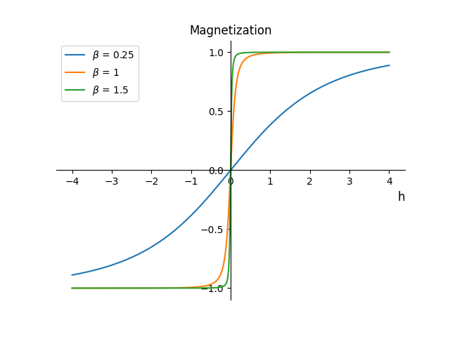
As shown in the above figure, in the lowest temperature where \(\beta = 1.5 \), the spin align perfectly to the external field. As the temperature goes up, the spin orientation becomes less susceptible to the external field.

Noting that \( M(H, T) \) being an analytic function for real \( H \) and non-zero positive \( T \). Meaning the physical and observable quantity in the system undergoes smooth transition with varing external magnetic field or change of temperature. One would expect a discontinuity in the material property if there is a phase transition. Hence, there will be no phase transitions in the case of the one dimensional Ising model.

Numerical Solution to 2D Ising Model

In two dimensions, we must consider both rows and columns in the lattice, introducing an additional index in the Hamiltonian:

$$ H = -J \sum_{(i,j)}\sigma_{i} \sigma_{j} - H \sum_{(i,k)}\sigma_{i} \sigma_{k} $$

With this in hand, the system could be broken down into canonical ensemble with a Boltzmann weight factor \( e^{-\beta E}(\beta = 1/k_{B}T) \) at the equilibrium temperature. Different from the one dimensional case, we will evolve the system state with probability governs by the Boltzmann weight factor for a particular temperature \( T \). Iterativelly carrying out this procedure bring the system to equilibrium state.

Then, given an observable \( A \) in a D-dimensional lattice with N identical spins localized on the lattice points, the average of the termodynamic observable \( A \) pertaining to this system in say the canonical ensemble is then given by

$$ \left< A \right> = \frac{\left[ \int{A(q, p)e^{-\beta E(q, p)}d^{DN}q d^{DN}p} \right]}{\left[ \int{e^{-\beta E(q, p)}d^{DN}qd^{DN}p} \right]}$$

However, numerical solution to the above many dimensional integral is quite impossible as for \( N \approx 10^{23} \). Resorting to Monte Carlo (MC) methods, the above equation turns into the simple unweighted average

$$ \left< A \right> = \frac{1}{M} \sum_{i=1}^{M} A(q_{i}) $$

where \( M \) is the number of microstates and \(\{ q_{i} \}\) refers to as a set of microstates, which is a subset of the ensemble.

The modified Monte Carlo scheme

In equilibrium statistical mechanics, an MC simulation uses pseudorandom number generators to sample the ensemble of the system according to the equilibrium probability distribution

$$ P(q^{\prime}) = \frac{e^{\beta E(q^{\prime})}}{\sum_{q} e^{-\beta E(q)}} $$

where the summation is carried out over all members of the set {\( q \)}, an MC simulation samples configurations (microstates) according to the Boltzmann weight factor \( e^{\beta E} \) and then weights them evenly.

The Metropolis algorithm

The Metropolis algorithm is a Markov chain Monte Carlo method for obtaining a sequence of random samples from a probability distribution if direct sampling is difficult.

Random walk in the sampling space, i.e, selecting a random microstate \(q^{\prime}\) from the set {\(q\)} with a probability distribution approaching \( P(q^{\prime}) \), is accomplished by the Metropolis algorithm. Using \( P(q) \) for two consecutives states \( q_{1}\) and \( q_{2}\) (the system moves from the former to the latter state in its phase space), it is obtained that

$$ \frac{P(q_{2})}{P(q_{1})} = e^{-\beta \left[ E(q_{2}) - E(q_{1}) \right]} = e^{- \beta \Delta E}$$

One important feature of this ratio is that it depends only on the energy difference between any two states, therefore, there is no need to have energies of all the microstates as included in the denominator of \( \left< A \right> = \frac{\left[ \int{A(q, p)e^{-\beta E(q, p)}d^{DN}q d^{DN}p} \right]}{\left[ \int{e^{-\beta E(q, p)}d^{DN}qd^{DN}p} \right]} \).

The Metropolis algorithm is accomplished in the following five steps:

• Step I. Change the present microstate \( q \) of the system to another randomly chosen state \( q^{\prime} \). In an Ising problem, this is equivalent to flipping a randomly selected spin. Since the total energy (E) explicitly appears in the Boltzmann weight factor, it must then be an explicit function of the microstate of the system in a way that change in q directly changes E.

• Step II. Calculate the energy difference \( \Delta E = E(q^{\prime} = E(q)) \)

• Step III. Perform steps I and II once for each spin in the system. The spins are usually selected randomly to ensure detailed balance. Steps I through III also define one MC sweep.

• Step IV. Repeat steps I through III for a number of MC sweeps in order for the entire system to be equilibrated. This value cannot be indeed estimated a priori. As a result, for an arbitrary value of temperature in the temperature loop of the code, one has to plot the total energy of the system at each step of equilibration and then check whether convergence is achieved.

Ergodicity

How can we make sure that the algorithm does indeed approach to a equilibrium state? Meaning we will stop the algorithm to update its state some point in time. Eqiulibrium as in the time averages of the system is equal to the ensemble averages of the system for time long enough, One criteria to check rather a particular algorithm eventually approaches equilibrium is the concept of ergdicity. By ergodic theorem, there are serveral conditions that need to be met in order to guarantee a equilibrium. However, in this case we just run the program and hope for the best.

Result

By running the algorithm with the following specification

L = 20         # Size of the square lattice
mcstp = 2000   # Number of MC sweep
eqstp = 2000   # Number of MC sweep for equilibration
D = 2          # Lattice dimension
N = L ** D     # Number of spins
NN = 4         # Number of nearest-neighbors
T_0 = 0.5      # Initial temperature
T_f = 10.0     # Final temperature
dT = 0.005     # Temperature step

We visualize four system properties as we vary the temperature in ratio of the critical temperature \( T_{c} \).

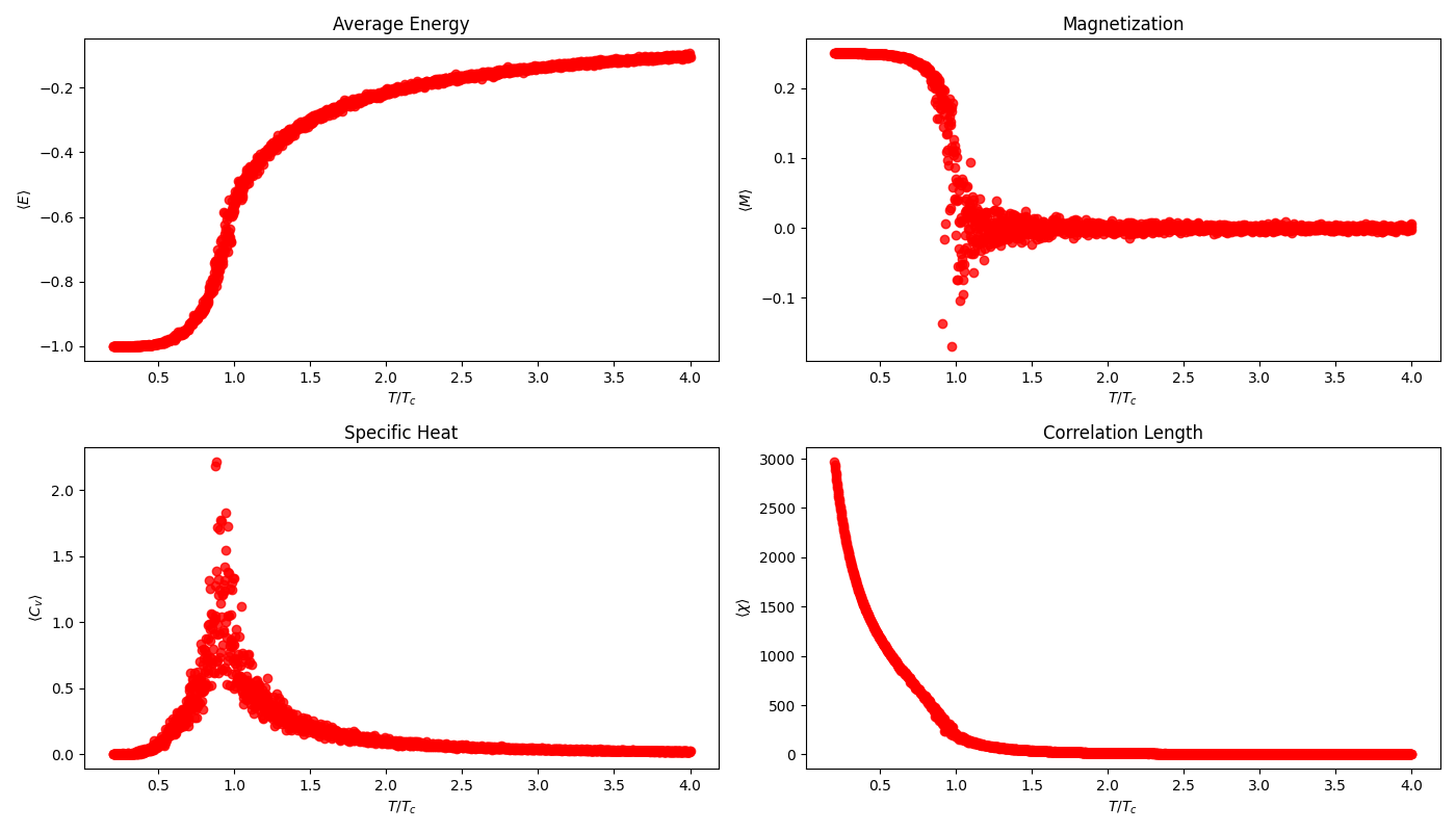
As shown in the graphs, all four properties demonstrated a sharp transition at \( T = T_{c} \). Clearly there is a phase transition at \( T_{c} \) for the two dimensional Ising model. At critical temperature, the material losses its magnetization and the correlation length drops to zero. To take in more energy to sustain the phase transition, the specific heat also raises at the critical temperature.

Final Remarks

As claimed ealier in this blog and what we have shown, there is no phase transition in the one dimensional Ising Model. In fact, Ising, being first one to solve the model further concluded that there will be no phase transition in arbitrary dimension. However, we known that it is not true seeing the extensive application of Ising Model on higher dimensional space in various field of science.

Another interesting aspect that’s worthy of further exploration is that what roles do dimensionality play in phase transition. From the isng model example, a new degree of freedom will lead to a emergent property that was no seen in the old system. It could be due to the change of topology as we increase the degree of freedom in the interaction but that’s another topics in another day. (For more information, one could check out ( Citation: Jalal, Khare & al., 2016 Jalal, S., Khare, R. & Lal, S. (2016). Topological transitions in ising models. Retrieved from http://arxiv.org/abs/1610.09845 ) )

Bibliography

- Ridderstolpe (n.d.)
- Ridderstolpe, L. (n.d.). Exact Solutions of the Ising Model. Retrieved from https://www.diva-portal.org/smash/get/diva2:1139470/FULLTEXT01.pdf
- Ashkan Shekaari (2021)
- Ashkan Shekaari, M. (2021). Theory and simulation of the ising model.
- Jalal, Khare & Lal (2016)
- Jalal, S., Khare, R. & Lal, S. (2016). Topological transitions in ising models. Retrieved from http://arxiv.org/abs/1610.09845
- (N.A.) (2021)
- (N.A.). (2021). Metropolis-hastings algorithm. Retrieved from https://en.wikipedia.org/wiki/Metropolis%E2%80%93Hastings_algorithm